Creating Kaplan-Meier Survival Plots with tflmetaR and gridify

Introduction

This vignette demonstrates how to create publication-quality Kaplan-Meier survival plots using the survminer package for visualization, gridify for professional annotation layouts, and tflmetaR for centralized metadata management.

The workflow covers:

Loading and preparing ADTTE (Time-to-Event) data from CDISC-compliant datasets
Fitting survival models and generating Kaplan-Meier curves
Combining survival plots with risk tables
Annotating figures with headers, titles, and footnotes using gridify
Integrating tflmetaR to pull annotations from external metadata files

Loading Required Packages

We begin by loading all necessary packages for survival analysis, data manipulation, and figure annotation.

library(tflmetaR)
library(gridify)
library(haven)
library(dplyr)
library(survival)
library(survminer)

Loading and Preparing ADTTE Data

The Analysis Dataset for Time-to-Event (ADTTE) follows CDISC ADaM standards. Here we use a synthetic oncology dataset generated by the CDISC Dataset Generator, containing 3 treatment arms and 500 subjects.

# get addtte data ----
# synthetic adtte for oncology therapeutic area from CDISC

adtte <- read_xpt(system.file("extdata", "adam_adtte.xpt", package = "tflmetaR"))

Data Transformation

We filter the data for Progression-Free Survival (PFS) analysis and prepare it for survival modeling.

tte <- adtte |>
  rename(avalc = AVALU) |>
  rename_with(tolower) |>
  filter(paramcd == "PFS") |>
  arrange(desc(trtp)) |>
  relocate(usubjid, trtp, cnsr, evntdesc, avalc, aval, trta) |>
  select(usubjid, trtp, cnsr, evntdesc, avalc, aval, trta)

tte$trtp <- factor(tte$trtp)

Fitting the Survival Model

We create a survival object and fit a Kaplan-Meier model stratified by treatment group (trtp).

# run survival modal ----
surv_object <- Surv(time = tte$aval, event = tte$cnsr)
fit1 <- survfit(surv_object ~ trtp, data = tte)

Creating the Survival Plot

The survminer package provides ggsurvplot() for creating publication-ready Kaplan-Meier curves with integrated risk tables, p-values, and median survival lines.

# survial plot and table ----
ggsurv <- ggsurvplot(fit1,
  data = tte, risk.table = TRUE, size = 1, # line size
  pval = TRUE,
  pval.size = 4,
  pval.method = TRUE,
  pval.method.size = 3,
  fontsize = 3,
  surv.median.line = "hv",
  tables.theme = theme_survminer() +
    theme(
      axis.text.x = element_text(size = 9, color = "gray30"),
      axis.text.y = element_text(size = 9, color = "gray30"),
      plot.title = element_text(size = 9),
      element_text(size = 9, color = "red")
    )
)

Customizing the Risk Table

We modify the risk table labels to display treatment group names in a more readable format.

# risk table -----
t <- ggsurv$table +
  scale_y_discrete(label = c("Treatment 3", "Treatment 2", "Treatment 1"))

p1 <- ggsurvplot(fit1, data = tte, risk.table = TRUE) ## can not add to the gridify directly

Combining Plot and Risk Table

Using ggpubr::ggarrange(), we combine the survival plot and risk table into a single figure with proper alignment and proportions.

# ggrance the survival plot  and risk table ----
p1 <- ggarrange(
  ggsurv$plot + labs(x = "", y = "Survival Probability") +
    scale_color_discrete() +
    theme(
      axis.title.x = element_text(vjust = 0, size = 9),
      axis.title.y = element_text(vjust = -3, size = 9), # y axis label
      axis.text.y = element_text(size = 9, color = "gray30"), # tick values
      axis.text.x = element_text(size = 9, color = "gray30"),
      legend.title = element_blank()
    ),
  t + labs(y = "") +
    theme(
      axis.title.x = element_text(vjust = 0, size = 9),
      axis.text.x = element_text(size = 9, color = "gray30")
    ),
  heights = c(2, 1.0),
  ncol = 1, nrow = 2, align = "v"
)

Annotating with gridify

The gridify package provides a framework for adding professional annotations to figures, including headers, titles, footnotes, and page numbers. The pharma_layout_base() function creates a layout compliant with pharmaceutical industry standards.

Basic Gridify Example

This example demonstrates manual annotation using gridify::set_cell() to populate each annotation field.

## --- use gridify to annotate the figure ---
fig <- gridify(
  p1,
  layout = pharma_layout_base(
    margin = grid::unit(c(1, 1, 1.23, 1), "inches"),
    global_gpar = grid::gpar(fontfamily = "Courier")
  )
) |>
  set_cell("header_left_1", "UCB") |>
  set_cell("header_left_2", "Drug X / Unspecified") |>
  set_cell("header_left_3", "STUDY001") |>
  set_cell("header_right_1", "CONFIDENTIAL") |>
  set_cell("header_right_2", "Final") |>
  set_cell("header_right_3", paste0("Data Cut-Off Date")) |>
  set_cell("output_num", "Figure F01") |>
  set_cell("title_1", "The Kaplan-Meier Curves of Progression-Free Survival Among Treatment Groups") |>
  set_cell("title_2", "Population: Safety Set") |>
  set_cell("title_3", "") |>
  set_cell(
    "note",
    paste0(
      "The synthetic oncology ADTTE was generated by CDISC Dataset Generator, ",
      "with 3 treatment arms and 500 subjects.\n",
      "Note: The Kaplan-Meier estimate of survival probability at a given time ",
      "is the product of these conditional probabilities up until that given time."
    ),
    mchar = 132
  ) |>
  set_cell("footer_left", "Program: f_surv_gridify.R, Source(s): ADTTE") |>
  set_cell("footer_right", paste0("Page ", 1, " of ", 1))

print(fig)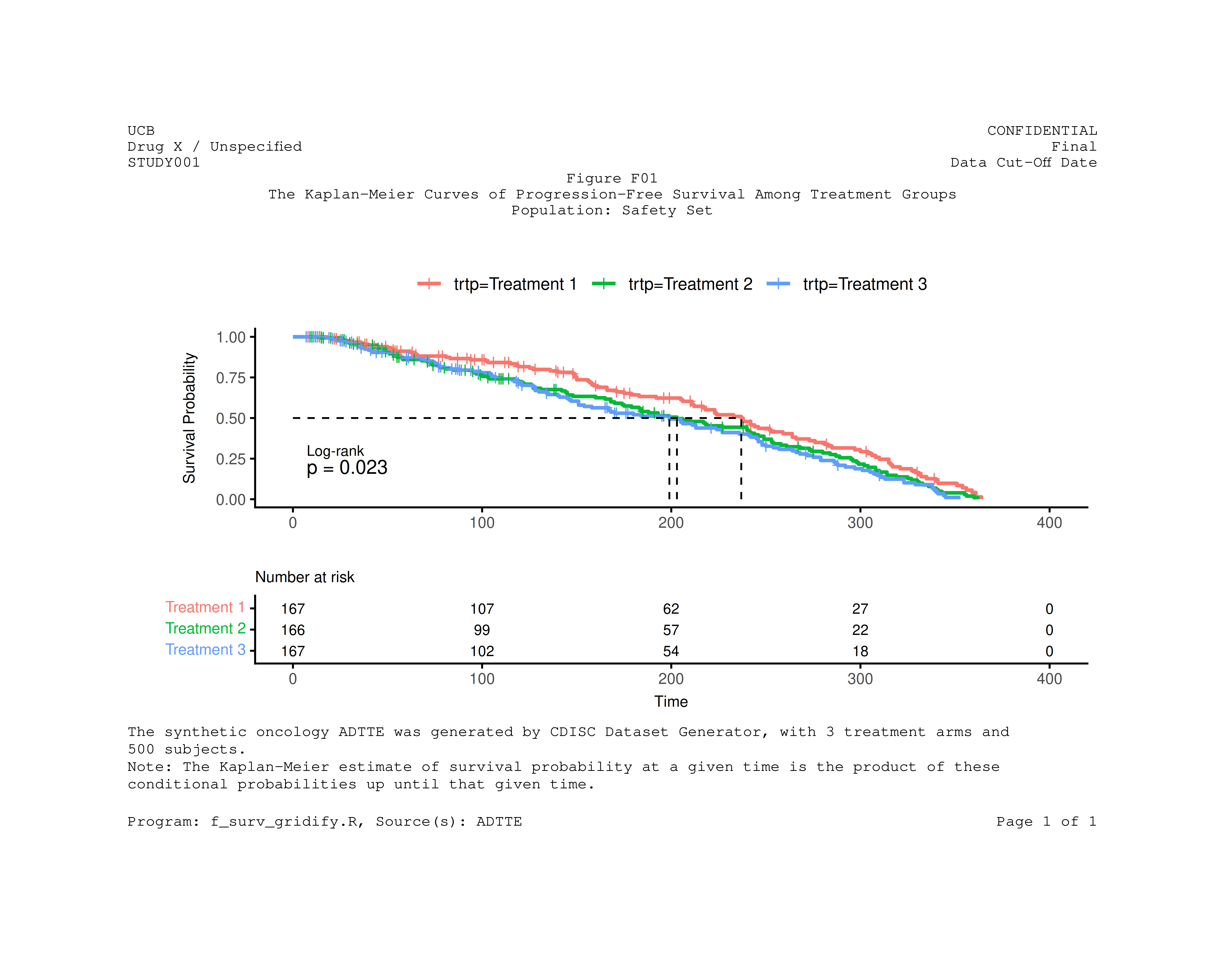

Integrating tflmetaR for Metadata Management

The tflmetaR package enables separation of metadata and code by storing titles, footnotes, and headers in external spreadsheets. This approach:

Centralizes all annotations in a single location to support audit and traceability
Reduces code complexity and maintenance burden
Supports regulatory compliance workflows

Loading Metadata Files

We read the titles and header information from an Excel spreadsheet.

## --- tflmetaR related code ----

# read headers, titles, and footnotes excel spreadsheet

file_name <- system.file("extdata", "st_titles.xls", package = "tflmetaR")
title_file <- tflmetaR::read_tfile(filename = file_name, sheetname = "Sheet1")
header_file <- tflmetaR::read_tfile(filename = file_name, sheetname = "Headr", validate = FALSE)

fig_number <- "Figure F01"

Extracting Annotations

Using tflmetaR accessor functions, we retrieve titles, footnotes, and header content for the specific figure.

ulheader <- tflmetaR::get_ulheader(header_file)[1, ]
urheader <- tflmetaR::get_urheader(header_file)[1, ]
titles <- tflmetaR::get_title(title_file, tnumber = fig_number)
footnotes <- tflmetaR::get_footnote(title_file, tnumber = fig_number, add_footr_tstamp = FALSE)
pgmname <- tflmetaR::get_pgmname(title_file, tnumber = fig_number)
source <- tflmetaR::get_source(title_file, tnumber = fig_number)

# convert footnote list to string
footnote_str <- paste(unlist(footnotes), collapse = "\n")

Creating the Final Annotated Figure

Now we combine gridify with tflmetaR-extracted metadata to create the final publication-ready figure. This approach ensures that any updates to titles or footnotes in the metadata spreadsheet are automatically reflected in the output.

## --- re-draw graph with pulled titles and footnotes ----
fig2 <- gridify(
  p1,
  layout = pharma_layout_base(
    margin = grid::unit(c(0.5, 1, 0.25, 1), "inches"),
    global_gpar = grid::gpar(fontfamily = "Courier")
  )
) |>
  set_cell("header_left_1", ulheader[[1]]) |>
  set_cell("header_left_2", ulheader[[2]]) |>
  set_cell("header_left_3", ulheader[[3]]) |>
  set_cell("header_right_1", urheader[[1]]) |>
  set_cell("header_right_2", urheader[[2]]) |>
  set_cell("header_right_3", urheader[[3]]) |>
  set_cell("output_num", titles[[1]]) |>
  set_cell("title_1", "") |>
  set_cell("title_2", titles[[2]]) |>
  set_cell("title_3", titles[[3]]) |>
  set_cell("note", footnote_str, mch = 120) |>
  set_cell("footer_left", paste0(
    "Program: ", pgmname, ",  ",
    "Source(s): ", source
  )) |>
  set_cell("footer_right", sprintf("Page %d of %d", 1, 1))

You can now preview the annotated figure or export the result to a PDF file using gridify::export_to(fig2, "f_surv_tflmetar.pdf").

print(fig2)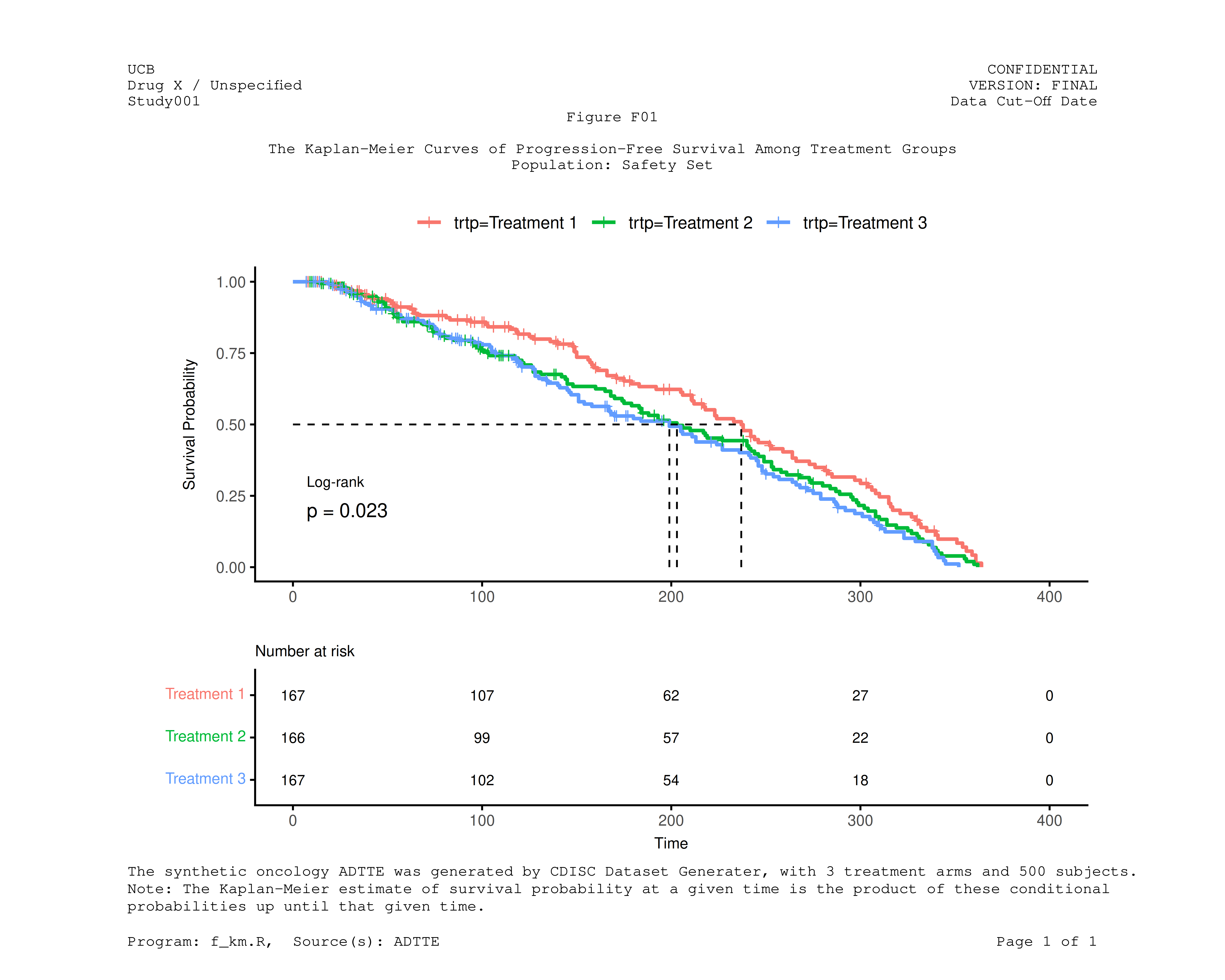

Summary

This vignette demonstrated a complete workflow for creating annotated Kaplan-Meier survival plots:

Data preparation: Loading and transforming ADTTE data following CDISC standards
Survival analysis: Fitting Kaplan-Meier models using the survival package
Visualization: Creating publication-quality plots with survminer
Annotation: Adding professional headers, titles, and footnotes using gridify
Metadata integration: Leveraging tflmetaR to externalize annotations for better maintainability

By combining these tools, organizations can produce regulatory-compliant figures while maintaining a clear separation between analysis code and presentation metadata.

Key Packages Used

Package	Purpose
`survival`	Survival analysis and Kaplan-Meier estimation
`survminer`	Publication-ready survival plots
`gridify`	Professional figure annotation layouts
`tflmetaR`	Centralized metadata management

tflmetaR Core Functions

Function	Description
`read_tfile()`	Read metadata from Excel or CSV
`get_title()`	Retrieve titles and subtitles
`get_footnote()`	Retrieve footnotes
`get_ulheader()`	Retrieve upper-left header content
`get_urheader()`	Retrieve upper-right header content